How to Do a Vlookup in Excel?

If you want to find a product in a database, you can use the vlookup function to find the data that most closely matches the lookup value. In this article, we will discuss using Wildcards in vlookup, and how to use the IFERROR function in front of vlookup to narrow down your search. If you have any questions, do not hesitate to contact us. We would be happy to answer your questions and help you use the Excel Vlookup function.
Using the vlookup function
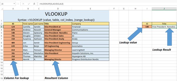
The VLOOKUP function searches the data in a cell range for the value that appears in the first column. If the value does not appear in this column, then VLOOKUP returns the next smaller value. However, it must be an exact match. If it is not, then VLOOKUP returns the wrong data. There are several ways to use VLOOKUP in Excel. This article will explain some of the most common uses for the function.
First, you must define the range of data to lookup. The range of data is defined by the column index number. This value can be a cell reference or a formula. In both cases, the ‘col_index_num’ argument specifies the column of data to search. The VLOOKUP function will return the closest value. It will return an error if there is no match. This function also allows you to use wild card characters to search for specific characters. You can also use an ampersand (&) to concatenate the lookup value on the fly.
Another way to use VLOOKUP is by using the =ROW() function. If you want to get the values of a helper column, you can use =ROW(). This function will return the row number in the cell. For example, if you need the value of a question mark, you can use =ROW(). If you want to get the values of the cell from a helper column, you can use the =ROW() function.
Another way to use VLOOKUP is to find things in a table. You can use this function to find the names of employees by row or column. By default, it returns an exact match. You can also use it to lookup values in other formats. You can try using INDEX, MATCH, or XLOOKUP functions instead. If you want to use VLOOKUP in Excel, you need a table with the columns in ascending order.
The VLOOKUP function looks up data in columns to the right of the matching value. You can also use wildcards to find partial matches. For example, if column A is the first column, then you would input =VLOOKUP(A6&D3) to find the next closest column in column D. However, the VLOOKUP function cannot look up values that are in columns at the same level as column A.
Wildcards in vlookup
If you need to search a list of names with a specific prefix, the asterisk wildcard symbol is your friend. This special symbol replaces multiple characters in the cell with a single character. The asterisk symbol is the easiest and most common way to search for the first name Riley. When searching a list of names, you can also use a cell reference. If the name Riley is spelled Riley, the cell reference is cell D2. However, it is important to understand that the value of this cell must be an exact match to the field being searched.
There are two types of wildcard symbols: the asterisk (*) and the question mark. The asterisk is more flexible than the question mark, but the question mark has fewer functions. Understanding how to use these characters in a VLOOKUP will save you from writing complicated formulas. This article will show you how to use the asterisk and question mark in a VLOOKUP.
The wildcard symbol can return multiple results if used in a VLOOKUP. In this case, the VLOOKUP will return the first match. For example, “Apple” would give the value for crabapple, but if you use *M??ts, you’ll get crabapple and apples. The same applies if you use ‘fishermans’ as a wildcard.
Another use of asterisk is replacing a character with a question mark. For instance, if the invoice number is P?inter, you’d type P?inter. However, the question mark is not an exact match, and the question mark replaces the asterisk by the tilde. The tilde character also nullifies the impact of wildcard characters. For this reason, wildcard characters should be avoided in most VLOOKUPs.
If you don’t have an exact match, you can use an asterisk (*) to filter the results. The asterisk is a wildcard that will search for any character between a string and a number of characters. It’s also possible to use asterisks in a vlookup that filter partial matches. This formula will give you the results you need. You can also use a tilde to nullify the impact of wildcards on the results.
Finding data that most closely matches lookup value
You may be interested in learning how to use VLOOKUP in Excel to find data that most closely matches a lookup value. While VLOOKUP is most commonly used to find an exact match, it can also be used to find a range of values. For example, you could find the price of a product by using the formula “Price:Konbu”; the result would be the product’s name and price. The data range would be A2 to B10.
The VLOOKUP function looks for data that most closely matches a lookup value. By default, it finds data that is the most similar or identical to a lookup value. If you have a list of web addresses, for example, you want to look up the URLs of each one of them. Some links begin with “https://,” while others do not. An approximate match will allow you to match the rest of the link while an exact match will prevent the VLOOKUP formula from returning errors.
In most cases, a VLOOKUP function will return a value in another column if the lookup value is equal or greater than the cell’s value. If the lookup value is less than or equal to the value of the cell, the “closest match” is the last cell in the lookup range. A table containing the values will be the last column in the lookup table.
The VLOOKUP function in Excel is a powerful tool for finding a unique value in a huge dataset. It is not a good idea to use Excel VLOOKUP in large data sets, but it is a good way to find the closest match. Practice the Excel VLOOKUP function by downloading a free template and practicing with it. Then, practice on it until you feel confident enough to use it on real data.
The VLOOKUP function in Excel works on a range-wise basis, so if one row has a higher value than another row, the result will be the higher row. But if the lookup value is a text value, it is more difficult to execute the lookup operation in Excel. For example, if the lookup value is “North Region Population,” the result would be “South Region Population.”
Using IFERROR function in front of vlookup
Sometimes you will see a #N/A error in the VLOOKUP formula. This error occurs because the formula cannot locate the value for the lookup. If you encounter this error, you should consider using the IFERROR function in front of VLOOKUP. The IFERROR function evaluates the result of VLOOKUP and replaces it with a custom value. This option is useful if you get a #N/A error as a result.
You can use IFERROR function in front of VLOOKUP to hide #N/A error. When VLOOKUP returns #N/A, the first IFERROR function traps the error. If the second or third VLOOKUP fails, the third IFERROR function catches the error and returns a message. If all Vlookups stumble, the last one will return a blank cell.
In this case, you can use IFERROR to catch errors caused by VLOOKUP formula. The IFERROR function will treat all errors produced by VLOOKUP formulas and functions. It will treat #NV errors, leading spaces, double spaces, and spelling errors. In addition to being able to trap errors, it will also allow you to use VLOOKUP formulas that require a cell reference.
The IFERROR function replaces the displayed error value with a custom message or another value. This prevents further calculations from being interrupted. This function can also catch #REF! errors, which happen when a cell reference is invalid. The result of this function will depend on how it is used. When you use VLOOKUP function, make sure to check the error message and the error value.
In order to use the IFERROR function in front of VLOOKUP, you should make sure that the last word in the formula is spelled correctly. Otherwise, it will result in an #N/A error. This error will result in a negative value. This problem can be solved by ensuring that the formula is error-free. There are some simple ways to use IFERROR in front of VLOOKUP.
The IFERROR function is a helpful function in Google Sheets. It works by detecting and replacing errors in formulas. The IFERROR function will return the original result, if it was correct. Alternatively, the blank cell will contain the original value. If you encounter an error, you can use the IFERROR function in front of VLOOKUP to create a more acceptable alternative.
We look forward to your comments and stars under the topic. We thank you 🙂